Visual Taylor Series

I recently came across some elegant Taylor Series diagrams, created by Amie Wilkinson. To try the technique myself, I made interactive versions. Here’s how to take them for a spin.

(If you ended up on this page but have never seen Taylor series: they’re a beautiful part of calculus. See this Khan Academy intro if you’re curious.)

1. A geometric series

As a warm-up, start with a simple, classic Taylor series: \( \dfrac{1}{1 - z} = 1 + z + z^2 + z^3 + \ldots \)

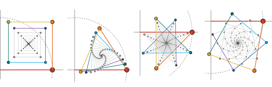
Move the black dot in the first diagram to define a value of \( z \) in the complex plane. As the value changes, you’ll see the partial sums of the series visualized in the second diagram. (On a phone? Scroll to see the second diagram. Also, you can touch next to the black dot so your finger doesn’t hide it.) The colors of the first few terms in the equation match the corresponding partial sums in the diagram.

The radius of convergence of the series is 1. If you keep the black dot in the dotted unit circle, you'll see the partial sums converge. If you move the black dot outside the circle, the partial sums will form a crazy, out-of-control spiral.

What happens at points right on or near the unit circle? Try it and see!

2. Complex logarithm: \( \ln (1 + z) \)

A closely related series yields the complex logarithm:

\( \ln (1 + z) = z - \dfrac{z^2}{2} + \dfrac{z^3}{3} - \dfrac{z^4}{4} + \ldots \)

Again, the radius of convergence is 1, and you’ll see a big difference for values of \( z \) inside and outside of the unit circle. But if you play with values right at the edge, you'll see some contrasts from the previous example.

A mathematical easter egg: what happens at \( z = i \)? It’s not a coincidence that \( 0.78 \approx \pi / 4 \). Read more here.

3. Complex exponential: \( e^z \)

Finally, let’s take a look at the complex exponential. \( e^z = 1 + z + \dfrac{z^2}{2!} + \dfrac{z^3}{3!} + \dfrac{z^4}{4!} + \ldots \)

Unlike the two previous examples, this series converges for all values of \( z \), thanks to the factorials in the coefficients. For any real value of \( z \), the infinite sum agrees with the value of raising the constant \( e \) to the power of \( z \). And for complex values of \( z \), this is a way to define the value of the expression \( e^z \).

Try moving the black dot along the vertical imaginary axis. You’ll see a right-angle spiral, always converging on the unit circle. At \( z = i \) you’ll see it converge at a special spot, a point at an angle of exactly one radian from the \(x\)-axis.

Notes

1. Numbers are rounded to two significant digits, and the implementation is not sophisticated. You may see arithmetic glitches, especially near the radius of convergence.

2. Sometimes when a series diverges the partial sums appear to be wheeling around a particular point. In these cases you might get the feeling that somehow averaging the sums would give a stable answer. This is one intuition behind the zoo of summation methods for divergent series.

3. The diagrams on this page all look something like spirals. That’s kind of a coincidence, not a general fact about Taylor series. It’s true, though, that any series with positive real coefficients will yield a spiral. There are a few other ways to guarantee a spiral, as the second example shows.

4. Someone on the original Twitter thread pointed to a 3Blue1Brown video with similar images. I don't know if this kind of diagram has name (maybe Wilkinson Diagram?) There’s also a whole separate genre of visualizations of Taylor polynomials converging.

5. The more I play with the exponential example, the more magical it seems that \( e^z \) is small when the real part of \( z \) has a large negative value. What a miracle of cancellation!